GIS
- QGIS
- GRASS
- SAGA
- ArcGIS
![]()
| Attribute | Desktop GIS (GUI) | R |
|---|---|---|
| Home disciplines | Geography | Computing, Statistics |
| Software focus | Graphical User Interface | Command line |
| Reproducibility | Minimal | Maximal |
GIS
Programming
They don’t work in isolation: API interfaces, and libraries / packages that enable interacting between programming languages (e.g. Rccp, reticulate, GDAL, GEOS)
Source: Lovelace, 2022
R is a language, has history, dialects and is evolving
spatial, sgeostat, splancs, akima, geoR, spatstats)spdep, compatibility with ESRI shape files maptools, handling coordinate referece systems rgdal, sp: interfaces with GDAL and PROJ libraries important today. gstat for spatio-tempral statistics, geosphere for spherical trigonometry, adehabitat for analysis of habitat selection in animals.sp: distinguishes spatial data from non-spatial objects, stores bounding box, CRS, but does not work well with raster.rgeos geometry operations (e.g. intersection)raster -> terra: map algebra, large out-of-memory datasets (interface with PostGIS)GRASS, spgrass6 rgrass7, RSAGA, RPyGeo, RQGIS, rqgisprocesssp, RGoogleMaps, ggmap, ggplot2, rasterViz, tmap, leaflet, rayshader, mapviewsf and terra actively developed. stars handles vector and raster data cubes, lidR processes airborne LiDAR (light detection and ranging) point clouds. rgdal, rgeos and maptools to be retired by end of 2023.Source: Lovelace, 2022 (Chapter 1)
Which one depens on your research question and data available
Vector
Raster
Most common packages today are sf and terra respectively
sf: simple features is an open standard endorsed by the Open Geospatial Consortium.
library(tidyverse)
library(sf)
system.file("gpkg/nc.gpkg", package="sf") |>
    read_sf() -> nc
nc.32119 <- st_transform(nc, 'EPSG:32119')
nc.32119 |>
    select(BIR74) |>
    plot(graticule = TRUE, axes = TRUE)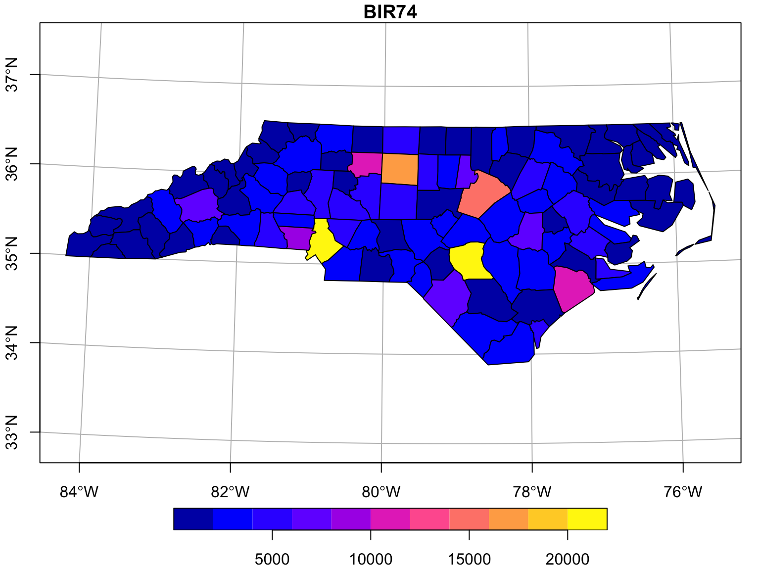
BIR74 is birth counts over the region (North Carolina)
| type | description |
|---|---|
POINT |
single point geometry |
MULTIPOINT |
set of points |
LINESTRING |
single linestring (two or more points connected by straight lines) |
MULTILINESTRING |
set of linestrings |
POLYGON |
exterior ring with zero or more inner rings, denoting holes |
MULTIPOLYGON |
set of polygons |
GEOMETRYCOLLECTION |
set of the geometries above |
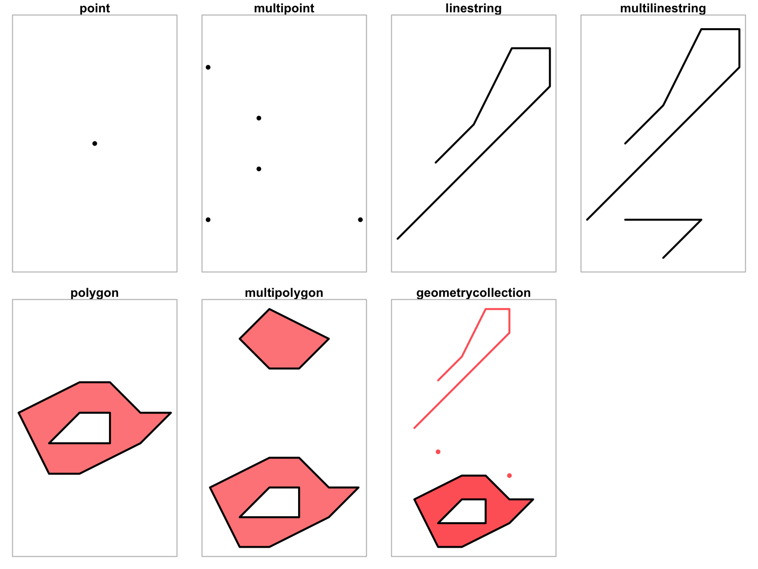
Other geometries include: CIRCULARSTRING, COMPOUNDCURVE, CURVEPOLYGON, MULTICURVE, MULTISURFACE, CURVE, SURFACE, TIN, TRIANGLE.
Source: Pebesma, 2022 (Chapter 3)
Simple feature collection with 100 features and 14 fields
Geometry type: MULTIPOLYGON
Dimension: XY
Bounding box: xmin: 123829 ymin: 14744.69 xmax: 930521.8 ymax: 318259.9
Projected CRS: NAD83 / North Carolina
# A tibble: 100 × 15
AREA PERIMETER CNTY_ CNTY_ID NAME FIPS FIPSNO CRESS…¹ BIR74 SID74 NWBIR74
* <dbl> <dbl> <dbl> <dbl> <chr> <chr> <dbl> <int> <dbl> <dbl> <dbl>
1 0.114 1.44 1825 1825 Ashe 37009 37009 5 1091 1 10
2 0.061 1.23 1827 1827 Alleg… 37005 37005 3 487 0 10
3 0.143 1.63 1828 1828 Surry 37171 37171 86 3188 5 208
4 0.07 2.97 1831 1831 Curri… 37053 37053 27 508 1 123
5 0.153 2.21 1832 1832 North… 37131 37131 66 1421 9 1066
6 0.097 1.67 1833 1833 Hertf… 37091 37091 46 1452 7 954
7 0.062 1.55 1834 1834 Camden 37029 37029 15 286 0 115
8 0.091 1.28 1835 1835 Gates 37073 37073 37 420 0 254
9 0.118 1.42 1836 1836 Warren 37185 37185 93 968 4 748
10 0.124 1.43 1837 1837 Stokes 37169 37169 85 1612 1 160
# … with 90 more rows, 4 more variables: BIR79 <dbl>, SID79 <dbl>,
# NWBIR79 <dbl>, geom <MULTIPOLYGON [m]>, and abbreviated variable name
# ¹CRESS_IDSimple feature collection with 100 features and 3 fields
Geometry type: MULTIPOLYGON
Dimension: XY
Bounding box: xmin: 123829 ymin: 14744.69 xmax: 930521.8 ymax: 318259.9
Projected CRS: NAD83 / North Carolina
# A tibble: 100 × 4
NAME AREA BIR74 geom
<chr> <dbl> <dbl> <MULTIPOLYGON [m]>
1 Ashe 0.114 1091 (((387344.8 278387.2, 381334.2 282773.7, 379438.2 28…
2 Alleghany 0.061 487 (((408601.8 292424.5, 408565.1 293985.3, 406642.9 29…
3 Surry 0.143 3188 (((478717.1 277490.3, 476935.7 278867.1, 471502.7 27…
4 Currituck 0.07 508 (((878193.9 289128.3, 877381.5 291117.1, 875993.9 29…
5 Northampton 0.153 1421 (((769835.3 277796.1, 768364.4 274841.8, 762615.8 27…
6 Hertford 0.097 1452 (((812328 277876.4, 791158.2 277011.9, 789882.3 2775…
7 Camden 0.062 286 (((878193.9 289128.3, 883270.9 275314.1, 881180.4 27…
8 Gates 0.091 420 (((828444.6 290095.5, 824767.5 287166, 820818.2 2871…
9 Warren 0.118 968 (((671747.1 278687.7, 674043.1 282237.4, 670407.8 31…
10 Stokes 0.124 1612 (((517436.7 277857.7, 479040.3 279098.1, 481102.2 31…
# … with 90 more rowsAn sf object looks like a data frame or tibble, but has a special geometry column
What they take as input
What they produce as output
TRUE| predicate | meaning | inverse of |
|---|---|---|
contains |
None of the points of A are outside B | within |
contains_properly |
A contains B and B has no points in common with the boundary of A | |
covers |
No points of B lie in the exterior of A | covered_by |
covered_by |
Inverse of covers |
|
crosses |
A and B have some but not all interior points in common | |
disjoint |
A and B have no points in common | intersects |
equals |
A and B are topologically equal: node order or number of nodes may differ; identical to A contains B AND A within B | |
equals_exact |
A and B are geometrically equal, and have identical node order | |
intersects |
A and B are not disjoint | disjoint |
is_within_distance |
A is closer to B than a given distance | |
within |
None of the points of B are outside A | contains |
touches |
A and B have at least one boundary point in common, but no interior points | |
overlaps |
A and B have some points in common; the dimension of these is identical to that of A and B | |
relate |
given a mask pattern, return whether A and B adhere to this pattern |
| measure | returns |
|---|---|
dimension |
0 for points, 1 for linear, 2 for polygons, possibly NA for empty geometries |
area |
the area of a geometry |
length |
the length of a linear geometry |
distance returns the distance between pairs of geometries.| transformer | returns a geometry |
|---|---|
centroid |
of type POINT with the geometry’s centroid |
buffer |
that is this larger (or smaller) than the input geometry, depending on the buffer size |
jitter |
that was moved in space a certain amount, using a bivariate uniform distribution |
wrap_dateline |
cut into pieces that do no longer cover or cross the dateline |
boundary |
with the boundary of the input geometry |
convex_hull |
that forms the convex hull of the input geometry |
line_merge |
after merging connecting LINESTRING elements of a MULTILINESTRING into longer LINESTRINGs. |
make_valid |
that is valid |
node |
with added nodes to linear geometries at intersections without a node; only works on individual linear geometries |
point_on_surface |
with a (arbitrary) point on a surface |
polygonize |
of type polygon, created from lines that form a closed ring |
segmentize |
a (linear) geometry with nodes at a given density or minimal distance |
simplify |
simplified by removing vertices/nodes (lines or polygons) |
split |
that has been split with a splitting linestring |
transform |
transformed or convert to a new coordinate reference system |
triangulate |
with Delauney triangulated polygon(s) |
voronoi |
with the Voronoi tessellation of an input geometry |
zm |
with removed or added Z and/or M coordinates |
collection_extract |
with subgeometries from a GEOMETRYCOLLECTION of a particular type |
cast |
that is converted to another type |
+ |
that is shifted over a given vector |
* |
that is multiplied by a scalar or matrix |
sfIntended to replace sp, rgeos, rgdal
tydiversesf objects have at least one geometry list column of class sfcsf objects starts with st_sfc objects have metadata:
crs: coordinate reference systembbox: bounding boxprecision attributen_empty: number of empty geometriesst_crs or st_set_crsCreation
library(sf)
# Linking to GEOS 3.10.2, GDAL 3.4.3, PROJ 8.2.1; sf_use_s2() is TRUE
p1 <- st_point(c(7.35, 52.42))
p2 <- st_point(c(7.22, 52.18))
p3 <- st_point(c(7.44, 52.19))
sfc <- st_sfc(list(p1, p2, p3), crs = 'OGC:CRS84')
st_sf(elev = c(33.2, 52.1, 81.2),
      marker = c("Id01", "Id02", "Id03"), geom = sfc)
Simple feature collection with 3 features and 2 fields
Geometry type: POINT
Dimension: XY
Bounding box: xmin: 7.22 ymin: 52.18 xmax: 7.44 ymax: 52.42
Geodetic CRS: WGS 84
elev marker geom
1 33.2 Id01 POINT (7.35 52.42)
2 52.1 Id02 POINT (7.22 52.18)
3 81.2 Id03 POINT (7.44 52.19)
sfheaders packages speeds-up the construction and manipulation of sf objects
sfReading & writing
Subsetting
Simple feature collection with 4 features and 5 fields
Geometry type: MULTIPOLYGON
Dimension:     XY
Bounding box:  xmin: -81.34754 ymin: 36.07282 xmax: -75.77316 ymax: 36.57286
Geodetic CRS:  NAD27
# A tibble: 4 × 6
  CNTY_ CNTY_ID NAME        FIPS  FIPSNO                                    geom
  <dbl>   <dbl> <chr>       <chr>  <dbl>                      <MULTIPOLYGON [°]>
1  1827    1827 Alleghany   37005  37005 (((-81.23989 36.36536, -81.24069 36.37…
2  1828    1828 Surry       37171  37171 (((-80.45634 36.24256, -80.47639 36.25…
3  1831    1831 Currituck   37053  37053 (((-76.00897 36.3196, -76.01735 36.337…
4 1832 1832 Northampton 37131 37131 (((-77.21767 36.24098, -77.23461 36.21…sftidyverse friendly:
tidyverse generics with methods for sf objects include filter, select, group_by, ungroup, mutate, transmute,rowwise, rename, slice, summarise, distinct, gather, pivot_longer,spread, nest, unnest, unite, separate, separate_rows,sample_n, and sample_frac.
If geometry to be removed:
st_drop_geometry()tibble ordata.frame before selectingsummarise method for sf
do_union (default TRUE) determines whether grouped geometries are unioned on return, so that they form a valid geometryis_coverage (default FALSE) in case the geometries grouped form a coverage (do not have overlaps), setting this to TRUE speeds up the unioningsffilter
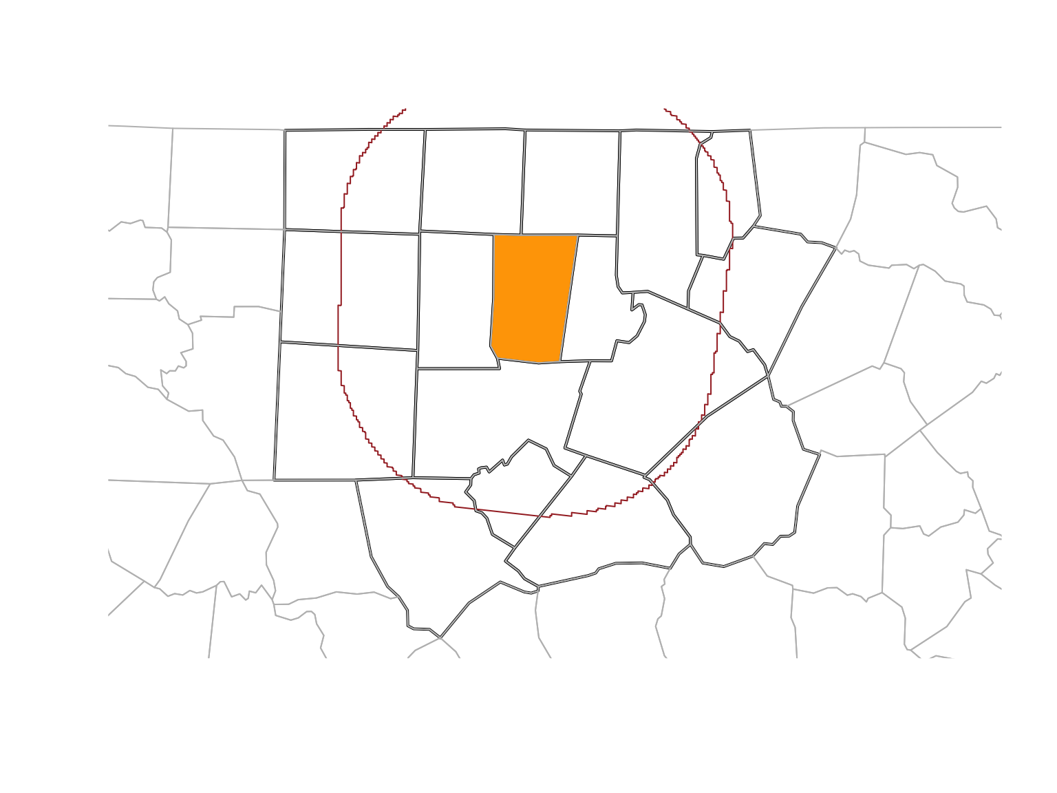
Select all counties less than 50 km away from Orange county:
orange <- nc |> dplyr::filter(NAME == "Orange")
wd <- st_is_within_distance(
    nc, orange,
    units::set_units(50, km))

o50 <- nc |> dplyr::filter(lengths(wd) > 0)
nrow(o50)
[1] 17Remember: The experession
::means accessing an object from a namespace (e.g. a function from a package)
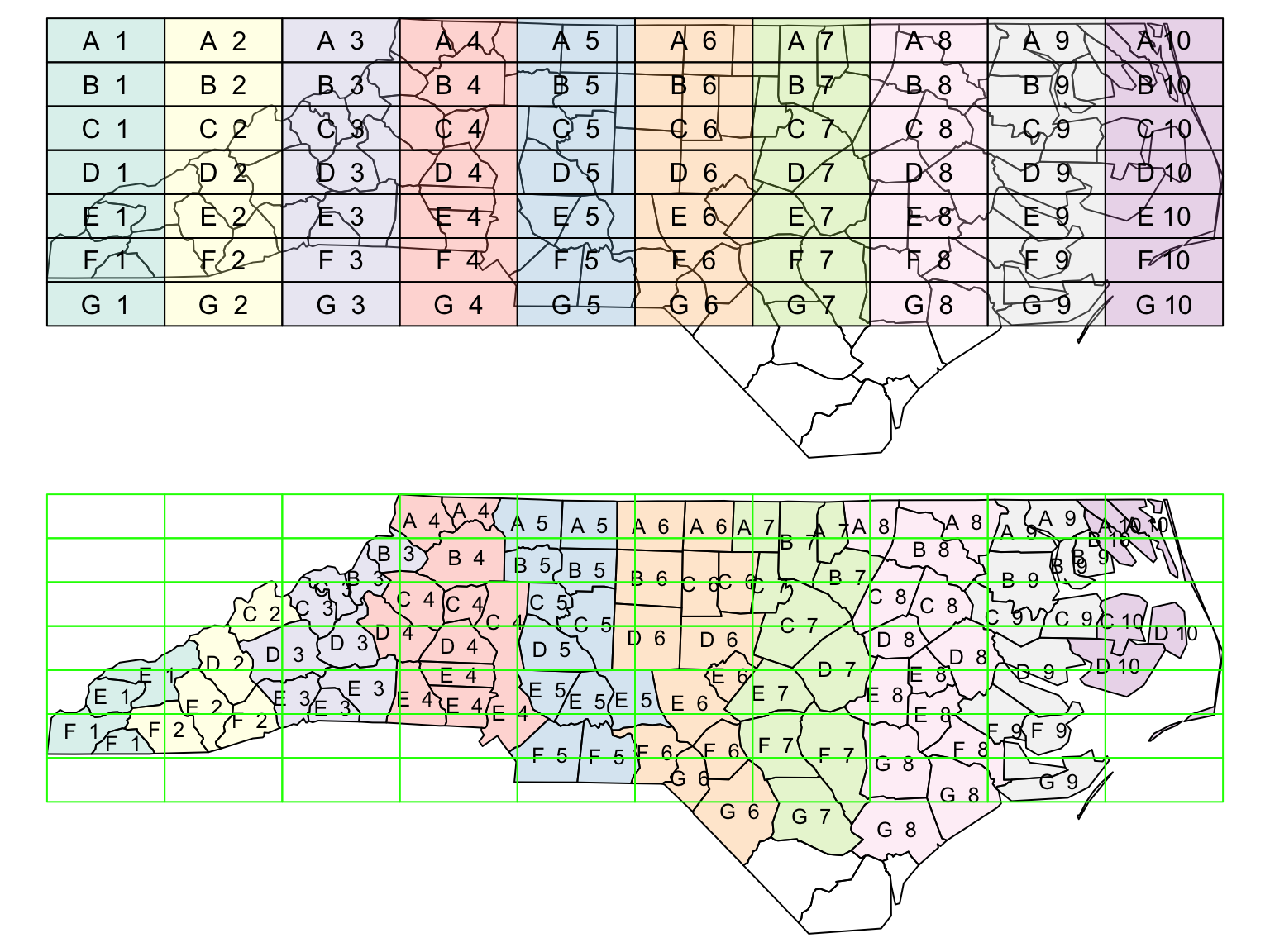
Work on spatial predicates instead of common columns. One needs to define spatially matching records
gr <- st_sf(
    label = apply(
        expand.grid(1:10, LETTERS[10:1])[,2:1], 1,
        paste0, collapse = " "),
    geom = st_make_grid(nc))

gr$col <- sf.colors(10, categorical = TRUE, alpha = .3)

# cut, to verify that NA's work out:
gr <- gr[-(1:30),]

# spatial join
suppressWarnings(nc_j <- st_join(nc, gr, largest = TRUE))

# graphics
par(mfrow = c(2,1), mar = rep(0,4))
plot(st_geometry(nc_j))
plot(st_geometry(gr), add = TRUE, col = gr$col)
text(st_coordinates(st_centroid(st_geometry(gr))), labels = gr$label)
# the joined dataset:
plot(st_geometry(nc_j), border = 'black', col = nc_j$col)
text(st_coordinates(st_centroid(st_geometry(nc_j))), labels = nc_j$label, cex = .8)
plot(st_geometry(gr), border = 'green', add = TRUE)
Example of largest = TRUE
sfSampling, gridding, interpolating:
st_sample: needs a target geometryst_make_grid: square, rectangular or hexagonal gridsst_interpolate_aw: area values to new areasCoordinate Reference System:
Know your CRS, transform when needed, and be careful when performing calculations on planar versus spherical geometries!
year_labels <- c(
    "SID74" = "1974 - 1978", "SID79" = "1979 - 1984")

nc_longer <- nc.32119 |>
    select(SID74, SID79) |>
    pivot_longer(starts_with("SID"))

## Ggplot friendly but needs long format
## objects to work with facets:

ggplot() +
    # geom_sf undestands special features!
    geom_sf(data = nc_longer, aes(fill = value)) +
    facet_wrap(~ name, ncol = 1,
               labeller = labeller(name = year_labels)) +
    scale_y_continuous(breaks = 34:36) +
    scale_fill_gradientn(colors = sf.colors(20)) +
    theme(panel.grid.major = element_line(color = "white"))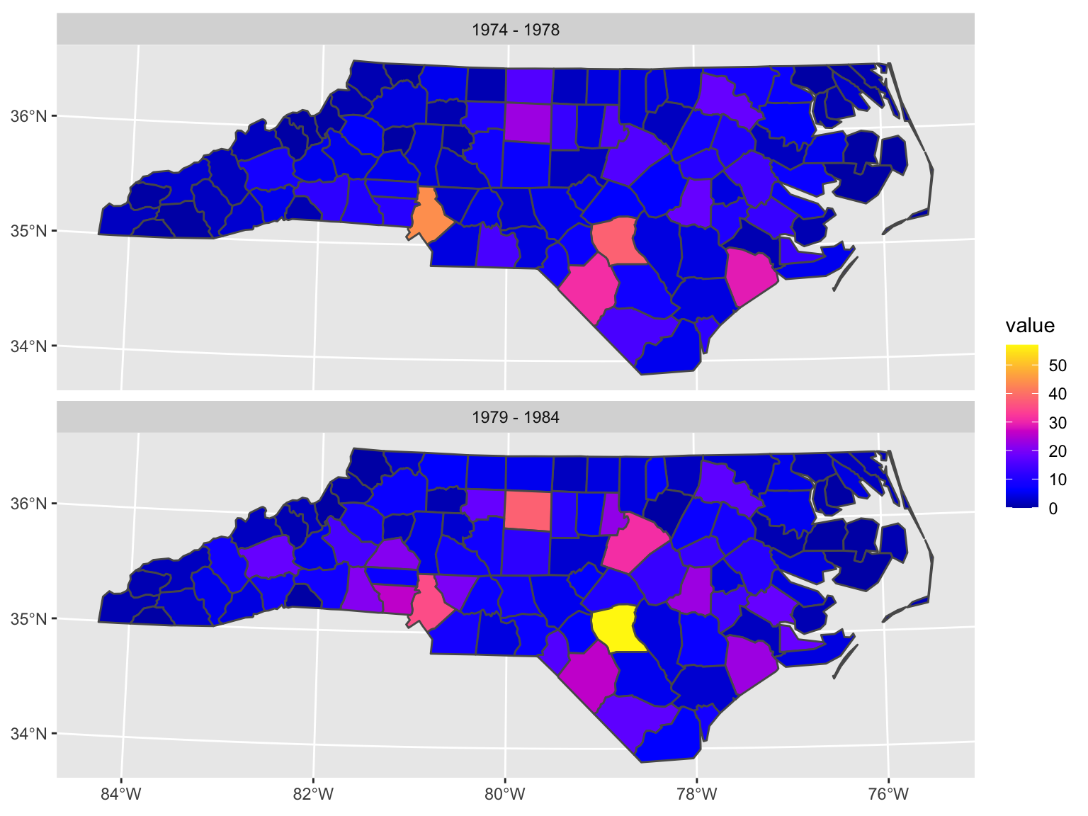
Lovelace, R; Nowosad, J; and Muenchow, J. 2022. Geocomputation with R. CRC Press
Pebesma, E; Bivand, R. 2022. Spatial Data Science
vignette(package = "sf") # see which vignettes are available
vignette("sf1") # an introduction to the package
vignette("sf2") # reading, writing and converting simple features
vignette("sf3") # manipulating simple feature geometries
vignette("sf4") # manipulating simple features
vignette("sf5") # plotting simple features
vignette("sf6") # miscellaneous long-form documentation
vignette("sf7") # spherical geometry operationsLow-hanging fruit
tmap, ggplot and mapviewTip: You need base map. Try map_data("world")
Challenge